Creating a Baseline for Our Version 2
Now that we have our R console of choice set up and have created a “Loading Page” for our R packages, we can create a new version of our dataset. From this new version, we will be able to add the new columns that will display the “Trip Distance” and “Day of Week”. Before we can do that, though, we’re going to need to set the current version of the dataset as a template from which we can build upon in R (I’ll be referring to this basic template as our “baseline”).
We’re going to want to create a new file and save it to the “R Desktop files” folder within our main “Marketing Analysis” folder. Since this file will create the basic format that we will want our dataset to be in, we will save this file as “Basic-Formatting-Page”.
This is a good point to introduce the concept of working directories, A working directory is the file location from which R will both upload and download datasets from. You can retrieve a spreadsheet from the set working directory, and you can also place a new spreadsheet (formed using R) into the working directory.
To see what your current working directory is set to, use the getwd() function. Simply type getwd() into the file and run that line of code. This will bring up the current working directory within the R console window.

Next, we will set our current working directory to the folder which has the data that we will be building up from (“Edited Data V1 CSV”). To change our working directory, we will use the setwd() function. Going back into R, type in setwd() within the “Basic-Formatting-Page” file as a new line of code, right underneath the line for getwd().
Within the parentheses of setwd() we will type in the file location of our “Edited Data V1 CSV” folder. The resulting line of code should look like this:
setwd(…/Marketing Analysis/Edited Trip Data 2021/Edited Data V1 CSV)
Now that we have set the working directory in the location of our latest spreadsheets, we can start to assign values in R for each of these sheets. We will use these values to edit the sheets using the R programming language. Since these will be new edits to the sheets, we will consider the results from our R code to be a new version, or “Version 2”.
Starting with the first the sheet for the first month in our dataset, we will make a value for the January sheet of Version 1 and call it “jan_21”. Whenever you want to assign a value to something in R, you just have to type in the name of that value and have that code chunk point to it. We can point a code of chunk to a value by using an arrow key and a hyphen to create a shape of an arrow. So if I type in: jan_21 <- , whatever is on the sending side of the arrow (<-) will be assigned our value (jan_21).
We’ll assign our “jan_21” value to our CSV file for January by using the read_csv() function. The read_csv() function is one of several functions included in the readr package. We should make sure to load readr from our loading page before proceeding.
This is a good time to note that there are several packages from that page that we should load by default, if we aren’t going to load every package on the page. The essential packages to load every time are namely: dplyr, tidyr, tidyverse, lubridate, and readr.
With readr loaded into our RGui workspace, we can assign the value of “jan_21” to our “2021-01-tripdata,csv” file, we will need to enter the following code:
jan_21 <- read_csv(“2021-01-tripdata.csv”)
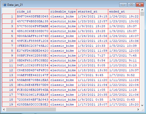
By typing up this code and then running it, we both bring the spreadsheet into the R workspace and assigned a name to it that we can call back to later (jan_21). To make sure that our line of code was successful, we can use the view() function to bring up the spreadsheet in R. Since the spreadsheet for January has been assigned to “jan_21”, we can view the sheet with the following code:
View(Jan_21)
Once we run this line of code, a new window should open up with the spreadsheet displayed in a basic format.

Now we know for certain that our spreadsheet for January is in the workspace and assigned to the desired value. Our “jan_21” value will serve as the baseline for our alterations to the spreadsheet. This means that we won’t want to actually change anything that falls within “jan_21”. In case we make a mistake, we want to be able to go back to “jan_21” and start over.
All of the changes here that we will be making to our dataset will be under Version 2. For January’s spreadsheet, we are going to want to create a new value for our second version. We’ll call this value “jan_21_v2”. We’ll assign this new value to equal the baseline that we set for our January spreadsheet, in order to build up the new version of the spreadsheet from there. Type in this line of code to assign the contents of our Version 1 into the contents of our fresh Version 2:
jan_21_v2 -> jan_21
After running this line, we will be able to pull up the same results with the view() function for both “jan_21″ and jan_21_v2”. To test this, go ahead and create a view() line for our Version 2 of January:
View(jan_21_v2)
This should bring up the same spreadsheet as before. With the baseline set for our Version 2, we should have a code chunk that looks like this.

We are going to want to replicate this code chunk for each month of the year. Once we have a Version 2 value assigned to every month in our 2021 dataset, we can move on to making the edits we want for our updated spreadsheets.