Data Visualization with R: Importing the Dataset

In the previous posts, we used SQL to organize the data that had been collected across the whole of 2021. We saved particular queries that offered useful insights into the story that our dataset provides. It’s time to turn these insights into visualizations, in order to will help our stakeholders understand the trends of the previous year.

To start off, we’re going to have to load up our library of packages from the Loading Page. In case you need a refresher, each line of code in our Loading Page should be ran in order to load in all the different R packages that we picked out to use for this project. Once you have run every line of code in the Loading Page, you will be ready to resume working in our R workspace.

The next step is to create a new file in R. Open a new script from the file tab in R menu and then save this file into the “R Desktop Files” subfolder of our Marketing Analysis folder. We’ll name the file “Plotting-Page”, because we will use it to plot out our data onto graphs.

As we did with our last R file, we are going to want to set our working directory as a folder. In this case, it will be the folder that is holding the SQL queries that we exported into CSV files for analysis.

Before we do this, however, it is best to check and see what directory the file is already set in. Run the getwd() line of code to see what the current working directory is for our file.

Once we have checked to see where the current directory is mapped, the next thing we will want to do is set the directory to be our 2021 SQL Queries subfolder. To do this, we should create a line in R that looks something like this:

setwd(“C:/Users/deanm/OneDrive/Desktop/Marketing Analysis/2021 SQL Queries”)

When we run this line, our R workspace will now pull files from and put files into the 2021 SQL Queries subfolder. Now we are ready to start assigning values to our spreadsheets.

We are going to write a read_csv() function in order to bring a file from our folder into our workspace. Starting with the file for our Classic Bike sheet, we would write our read_csv() command with the name of the file nested within it, like so:

read_csv(“all-year-2021-classic_bike.csv”)

This will bring our Classic Bike data into the workspace, but we will need to assign a value to it in order to call upon it later. Let’s assign it the value of “classic_bikes”. To do this, simply point the read_csv code towards the name we wish to give it. Your complete line of code should look like this:

classic_bikes <- read_csv(“all-year-2021-classic_bike.csv”)

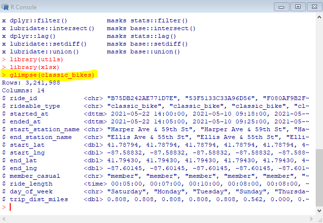
Run that line of code, and then use a glimpse() function to check the results. Nest the new value for our spreadsheet inside the function, like so:

glimpse(classic_bikes)

After running this glimpse() function, your R console window should look something like this:

Now repeat this process for all of the other csv files that you have put in this folder. Assign each file a value and then check to see that it has been loaded in properly.

With all of the desired SQL data now loaded up into R, we can begin writing code lines that will generate graphs of our data. These lines will start off simple enough, but can get more complex as we work towards perfecting our visualizations. We’ll go over the basics of this in our next post.