Finding the Mode and Expanding our Queries

In the last post, we went over the somewhat painstaking process of finding both the Max and Mean of our ride_length column. These are useful bits of information that we can use in our analysis and later on in our presentation . Another insightful bit of data that we can extract from our dataset is the Mode value of certain columns.

The Mode of a dataset (or in this case, column) is the value that comes up the most often. You might view the Mode as the most popular value. Given the type of values that we have throughout the dataset, we would only benefit from finding the Mode of certain columns.

For instance, we could find the Mode value for our start_station_name column, and that would tell us the most popular starting location amongst our riders. However, this information might not be as useful to helping us determine how causal riders use their bikes differently than members.

A much more useful application of the Mode value would be to find the most popular day of the week for our riders. We could see which day is the most popular amongst all riders, and then compare that to which is most popular amongst our causals and our members.

In order to find the Mode value of a column in our dataset in SQL, we will need to introduce some new functions to our queries. Namely, these are the TOP, ORDER BY, and GROUP BY functions.

The TOP function is used to find the highest values in a specified dataset. It can be used to bring up the top 1 row of a dataset or the top 1 million rows. The syntax for the TOP function is to write TOP after your SELECT statement and follow it by the number of rows that you want to display. Then, you place the name of the dataset (or column) immediately afterward. It also helps to follow this with an AS statement to give this value a name.

The ORDER BY and GROUP BY functions often work in conjunction to help us sort out the results of our query. We use GROUP BY to determine which column in our data will be used to determine the order of the rows. The ORDER BY function is used to specify by what criteria the data should be ordered by.

The syntax for both ORDER BY and GROUP BY are rather simple. Using GROUP BY first, we type GROUP BY and follow it with the name of the column that we wish to use to organize our data. Then in our ORDER BY statement, we would use the function that we will use to sort out the data, and follow that by what order we would wish for it to be queried in (ascending or descending order).

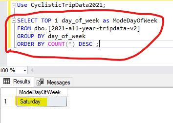
To find out what is the most popular day of the week, we would SELECT the TOP 1 row of the dataset (day_of_week). We would follow that with a FROM statement that calls up our all-year-v2 table. Next, we use GROUP BY and assign it to our day_of_week column. Finally, since we are going off of an overall count of days in the week that people decided to ride on, we end our query with an ORDER BY statement that uses the COUNT(*) function and puts our results in descending order (DESC).

Here is what our query should look like:

SELECT TOP 1 day_of_week as ModeDayOfWeek
FROM dbo.[2021-all-year-tripdata-v2]
GROUP BY day_of_week
ORDER BY COUNT(*) DESC ;

Remembering to us an AS statement to name our results “ModeDayOfWeek”, we should come up with the following results:

We can see here that the most popular day overall for our riders is Saturday. But what the most popular day for our members? How about the causal riders?

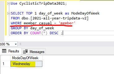
We can find the answer to both of these questions by inserting a simple WHERE statement into our query. To find the most popular day amongst members, we just need to place a WHERE statement directly after from, and specify that the member_casual value should equal ‘member’.

Here is what that query would look like:

As you can see, it was rather easy to find out that the most popular day amongst our members was Wednesday. We can make a similar query to find out the most popular day amongst our casual riders. Simply swap the ‘member’ value for the ‘casual’ value.

This can be replicated with our Max and Mean queries as well, just by adding a WHERE statement to them. We should make a comment above each of these queries, explaining what results they are meant to show. We’ll continue to explore the Mean, Max, and Mode of our data on a single file and save it as “ALL-YEAR-2021-max-mean-mode”.

One more route of analysis we can take with this file is ranking the popularity of days from most popular to least popular. We can find the results of this amongst our overall customer base, and then compare that to the results from our members and our causals.

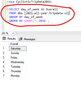
To rank the days by popularity, we can reuse the query that we wrote to find the Mode day of the week. All we would have to do is remove the “TOP 1” statement from that query. Be sure to keep “day_of_week” in the SELECT statement. That way, when the query is executed, all of the days will be listed in the order of which had the highest count in our dataset to which had the lowest. The query should look like this:

Now we know that Saturday is the most popular day, and Monday is the least. Go figure!

We should continue to gather metrics such as those above from our dataset. When we feel like we have enough of this summary information collected, we can export all of these queries as single CSV files, which we will be combining into a summary file in our next post.