Making Queries in SQL: SELECT, FROM, and WHERE

In the previous post, we were able to import our dataset by using the Data Import Wizard. During the process, we wrote some simple queries to create our database and to alter the data within it. Taking these steps set up our project to where we can now begin the Analysis Phase in earnest.

Our main strategy in this analysis will begin by using SQL to create filtered datasets that show what data meet certain criteria. We can gather some basic insights with this information and can also use the Data Export Wizard to bring some of our findings into CSV format. It’s from these CSV files that we will make visualizations (graphs and charts) of the data in R.

We’ve already gotten a small taste of what SQL queries can do in the last post. Those queries used very specialized SQL statements, which were made to do some of the more unique tasks that can be done for a dataset using the language. We will now focus on running some of the more basic queries that are essential for digging up information that will be useful to our analysis.

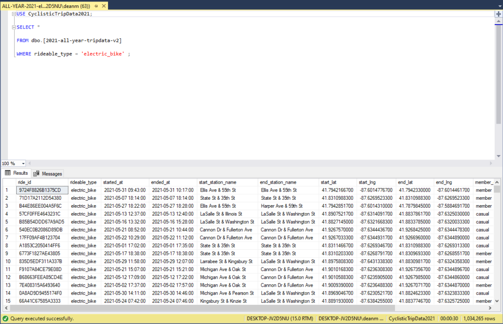
The goal of these queries is to create smaller datasets that are more focused on a particular aspect or range of our data. We can do this by using a basic combination of functions in SQL: SELECT, FROM, and WHERE. For example, to create a query that shows us all of the electric bike rentals throughout the year, we would create the query as follows:

Let’s break this query down one line at a time.

The SELECT statement is used to indicate what exact information we wish to extract from the table. This pertains to any column or group of columns from wish we want the query to draw information from. If we wish to pull up data from every column in the table, we use the asterisk symbol ( * ) right after SELECT.

The FROM statement is there to specify which table it is that we will be working with. All we have to do to use a FROM statement is to place the name of the table right after FROM. In SQL Server, we can type “dbo.” after FROM to bring up a dropdown menu where we can select the table that we wish to use. Remember that this will only happen if there is also a USE statement executed in the file that contains the name of the database to which the table belongs to (ex: USE CyclisticTripData2021 ; )

The WHERE statement is used to offer a condition or criteria that the data must meet in order for the query to pull it up. WHERE statements are structured using three elements, resembling a simple mathematical equations.

• First, we need to specify which column contains the data that we wish to use as a qualifier for the data brought up by our query.
• Second, we need to use a conditional symbol (known as an operator) to set the condition in which the data must qualify in order to be selected. There are several symbols to use here, and they correspond to what these symbols mean in mathematics. These operators include the equals sign ( = ), the less than sign ( < ), the greater than sign ( > ), and variations of these. To use an operator that negates one of the symbols mentioned above, we place an exclamation point ( ! ) in front of it (not-equals would be: != ). The “or equals to” operators are used by placing the equals sign behind another operator (less than or equal to would be: <= ).
• Third, we need to input the value which the WHERE statement will sort out based on the criteria made in the other two parts of the statement. This value should be something that is found within the column that we specified at the beginning of the statement. In the example above, the value ‘electric_bike’ is found within the column rideable_type. Note that we should always use single quotation marks ( ‘ ‘ ) around the value we are searching for.

When combining these elements for our sample query above, the results should look like this:

Using this basic combination of statements, we can set aside new subsets of data that we will analyze and visualize using other programs. We can do this for the other types of bikes as well (docked bikes and classic bikes), just to see if there are any interesting insights. After each of these queries, I went ahead and saved the file so it can be pulled up again later. For the electric_bike query that we just did, I named the file “ALL-YEAR-2021-electric_bike”.

It’s important to also try to find insights into specific values while we are making our SQL queries. 

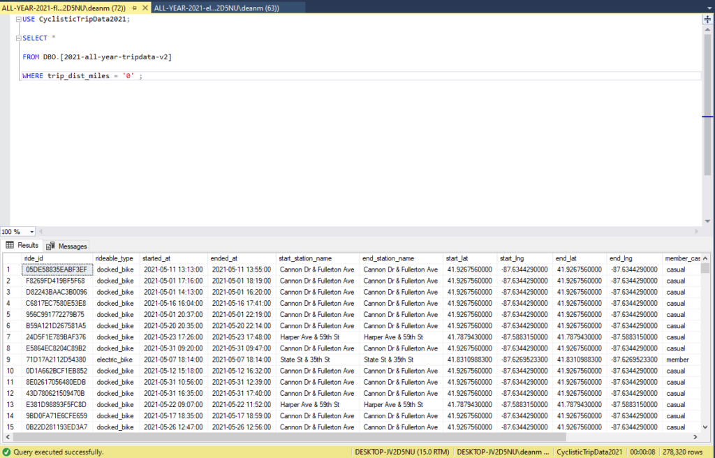
For example, if we dig into our trip_dist_miles column and query distances of 0 miles, we get some interesting results.

Here we see that there are thousands of riders whose data would pull up a “0” result. Most of them have significant ride times. It’s important to remember here that trip_dist_miles is based on the geospatial distance from the starting location and the ending location for each ride. If trip_dist_miles reads as “0” in a row, that just means that the rider returned the bike to the same station that they started their journey in.

These riders we will term “floaters”, because they are essentially hovering around the same area and will eventually land back in the same spot that they originated from. We’ll go ahead and save this query file as “ALL-YEAR-2021-floaters”.

It is also a good idea to recreate the quarters of the yearly data that we have uploaded into our SQL server. When we imported the dataset and adjusted the datatypes of each column to fit our analysis, we changed that data slightly from how it was in our original CSV sheets. Now, we should use a SQL query to create new spreadsheets with the current data types.  

The queries that we will be making for the quarters will be a bit more complex than the previous queries. We will still be using the SELECT FROM WHERE template, and will use a BETWEEN statement to specify what times our query results should be filtered between. We will also use an INTO statement to create new tables in our SQL Server database.

The BETWEEN statement is used to specify a range of values within a column, and it falls within the WHERE statement. The BETWEEN statement acts as an operator for the WHERE statement. After stating the column in our WHERE statement, we would type BETWEEN and enter the first value in our range. Next, we would type the AND statement to act a sort of operator for BETWEEN. Think of it grammatically, where you would say that something is “between” x “and” y. Finish the statement by putting the end value for the range. Also remember that you will be putting single quotation marks around the values in this statement.

The INTO statement is used to specify what table the data from your query is meant to be transferred into. It can simultaneously create a new table with the data from the query. To create a new table with our query data, type INTO on the line following your SELECT statement. Next, type in the name of the table that you wish to create. Be sure to put the table name behind the brackets of “dbo.[]” when you write it in the code. Also, make sure that the line that holds your INTO statement is between the SELECT and FROM statements.

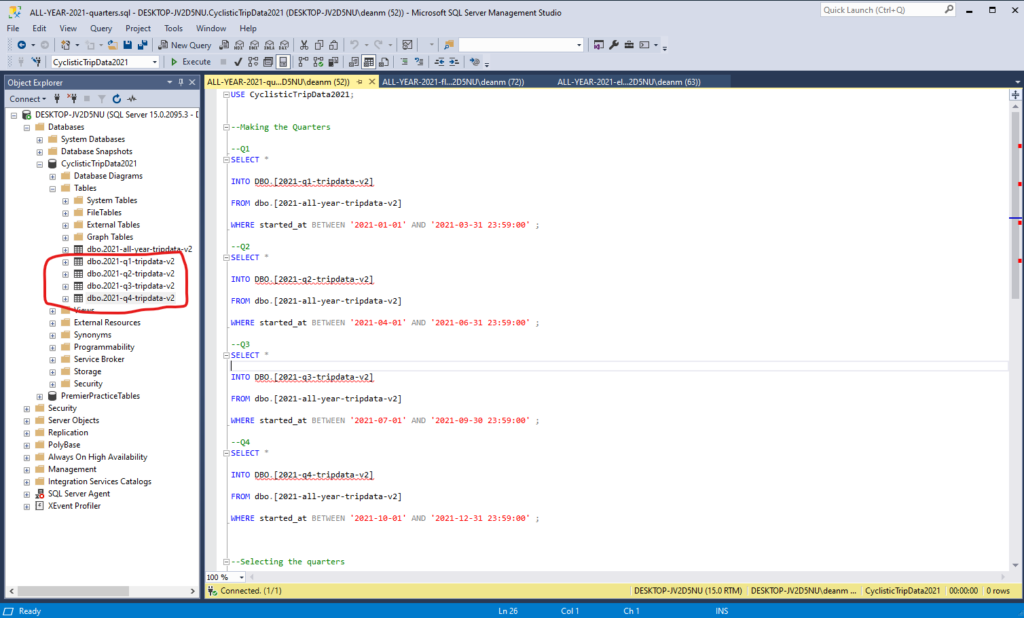
Your query for the first quarter should look like this:

Note that for the values used in our BETWEEN statement, the first value does not include a time value, while the second one has a time value of “23:59:00”. This is done because in the datetime datatype, a value that only has the date will automatically be assigned a time of “00:00:00”, which is 12:00 AM. The end value for our range needs to have the time specified to the last minute of that day, hence “23:59:00” stands in for 11:59 PM. The seconds value here is “00” because our dataset does not include time in seconds.

With this understanding of how to make new tables for our quarters using the INTO and BETWEEN statements, we can move forward with creating a table for all four quarters. We will keep the “V2” designation for our dataset when naming these new quarter tables, because the alterations we made to the table are only for the purposes of using SQL efficiently, and the data remains much the same. Use the naming convention “dbo.[2021-q1-tripdata-v2]” for each of the quarter tables.

After writing the queries for each new quarter table, write a SELECT * statement for each of them in order to use the Export Wizard to turn them into CSV files later on. For now, save the file with all these new table queries as “ALL-YEAR-2021-quarters”. The finished file should look something like this:

At this point, we have covered the fundamentals of the SQL queries that we will be making in our analysis. In the next post, we will dig a little deeper into the data and use these basic SQL statements to help us continue to explore it.