Downloading New Sheets for Version 2
We just did a lot of heaving lifting in our R workspace, creating new columns using several nested functions. Now that we have completed adding the three additional columns to all 12 of our spreadsheets for 2021, we can move on to combining these spreadsheets and saving them to new ones.
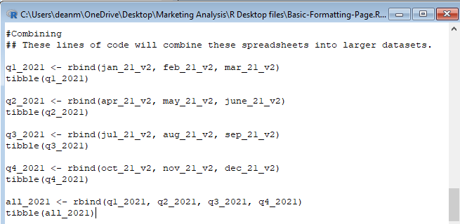
We will combine these spreadsheets into the four quarterly tables, and then combine the quarters into a dataset that shows the entire year of 2021. To combine our current datasets into quarters, we will use the rbind() function.
Starting off with the first quarter. place the names of the tables you wish to combine (ex. jan_21_v2, feb_21_v2, mar_21_v2) into the rbind() function and assign them the name q1_2021. You’re resulting line of code should look like this:
q1_2021 <- rbind(jan_21_v2, feb_21_v2, mar_21_v2)
This will result in a large dataset that we have assigned the value of q1_2021. To make sure that the data has combined correctly, we can either use a View() to see the entire spreadsheet, or we can use a tibble() function to get a preview of the dataset in the R console window. We use tibble() in the same way as view(), by inserting the desired value into the function:
tibble(q1_2021)
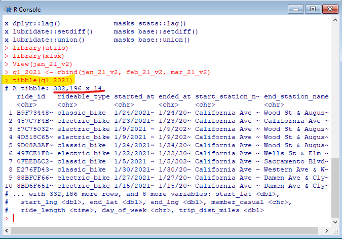
Running this line of code should bring up this result in the R console window:

Note that the the first line of the tibble() preview will show how many rows of data there are, and how many columns. You can use this knowledge and compare it to that of the datasets which you have combined to confirm if the new value of q1_2021 was made correctly using rbind().
Do the same for the other three quarters, matching each quarter with the tables that correspond to the months that fall under it. Once you have all four quarters bound and declared, you can use the rbind() function once again to combine them into a table for the whole year. Name the table “all_2021”. You should now have five new dataset values to work with: q1_2021, q2_2021, q3_2021, q4_2021, and all_2021.

With all of our desired datasets assigned values in our R workspace, the final step in R is to download these new tables into spreadsheets that we will use in our analysis. For this, we will use the write_csv() function.
The write_csv() function will create a new CSV file and place it in our working directory. To do this, we simply nest the name of the value we wish to turn into a CSV file, and the we follow it by what we wish to name the file in quotation marks.
Before I show you an example of a write_csv function, it’s important for us to remember that we will want to put these new files into a folder made specifically for our Version 2 dataset. We should make a subfolder in “Edited Trip Data 2021” and call it “Edited Data V2”. Once we have that folder made, we’ll make it our working directory in our R workspace.
Your setwd() code should look something like this:
setwd(“…/Marketing Analysis/2021 Edited Trip Data/Edited Data V2”)
Once we’ve set “Edited Data V2” as our working directory, it will become the destination of our new CSV files that will be made using write_csv(). We’ll start with our January file for Version 2. Using the value of jan_21_v2, our write_csv() code should look like this:
write_csv(jan_21_v2, “2021-01-tripdata-v2.csv”)
Note that the naming convention that we’re using for the file is the same as with our original, raw spreadsheets. The only difference is the “v2” added at the end of the name, for Version 2. We will use this convention for all of the monthly tables. For our new quarterly and yearly tables, we can put the timeframe information at the front of the file name, where the date would be. For example, Q1 2021 would be named “q1-2021-tripdata-v2.csv”.
Make a CSV file for all 12 of our monthly tables, then do the same to the four quarterly tables as well as the yearly table for 2021. We now have CSV files saved for all of the tables that we have worked on in R.
There is one last step we should take before diving into a deeper analysis of our data. We should upload our yearly dataset into a platform that can handle such a high volume of information.
The data in ‘2021-all-year-tripdata-v2.csv’ is going to have well over 4.5 million rows! This is well over the limit that Excel is capable of processing. If we were to open this csv file using Excel, the file would cut the data off at around 1 million rows, and all the rest of our data would be lost.
To work around this, we will use a free extension to Python known as ‘Mito’, which can be used to work with an unlimited amount of data. To use Mito, we will first need to install Python and create a Jupyter Notebook within an Anaconda environment.
All of that may sound like gibberish to anyone who is unfamiliar with Python and it’s various extensions. That’s fine, because this is not a major part of the project and can be skipped over. This would just be a safe practice to have if this were for a job, because such a large dataset should have a backup in which it can be viewed in it’s entirety.
If you are going to back up your dataset using Mito, you’ll first need to follow these tutorials for setting up a Jupyter Notebook using Python and Anaconda.
- Python: https://phoenixnap.com/kb/how-to-install-python-3-windows
- Jupyter Notebook & Anaconda: https://www.dataquest.io/blog/jupyter-notebook-tutorial/
Once you are able to make an environment in Jupyter Notebook, it’s time to set up Mito. Here is a tutorial on how to install Mito.
With Mito up and running, we can import our spreadsheet into the virtual environment we just created. This will be useful if we want to work on this data in the future using spreadsheet functions. At the very least, its a safe place to store our yearly data. We are now ready to finish up the “Process” Phase of our project and go into the most critical phase: Analysis.